The Pwned Password data set contains 551,509,767 sha1 hashes from passwords exposed in data breaches. Troy Hunt has provided an API for searching this data, but interacting with a third-party service is not always an option. A third-party service may have concerns about privacy, availability, and reliability. The size of the data set makes it difficult to include in a web application, just the hashes are about 21 GB. I spent some time investigating what is required to package this data as a SQLite database and as a bloom filter for the JVM.
SQLite Database
Each data point contains a sha1 hash and the number of times that password appeared in a breach
➜ head pwned-passwords-sha1-ordered-by-hash-v4.txt
000000005AD76BD555C1D6D771DE417A4B87E4B4:4
00000000A8DAE4228F821FB418F59826079BF368:2
00000000DD7F2A1C68A35673713783CA390C9E93:630
00000001E225B908BAC31C56DB04D892E47536E0:5
00000006BAB7FC3113AA73DE3589630FC08218E7:2
00000008CD1806EB7B9B46A8F87690B2AC16F617:3
0000000A0E3B9F25FF41DE4B5AC238C2D545C7A8:15
0000000A1D4B746FAA3FD526FF6D5BC8052FDB38:16
0000000CAEF405439D57847A8657218C618160B2:15
0000000FC1C08E6454BED24F463EA2129E254D43:40
I removed the number of occurrences to reduce the size of the data set and speed up subsequent commands
➜  time sed -i '' -e 's/:.*$//g' pwned-passwords-sha1-ordered-by-hash-v4.txt
sed -i '' -e 's/:.*$//g' pwned-passwords-sha1-ordered-by-hash-v4.txt  1497.24s user 110.03s system 93% cpu 28:40.04 total
➜
Creating the SQLite database was very simple with the built in .import command. This command will insert each line in a file into a table, so no custom script is necessary. Just the following four commands creates the database and schema, inserts the data, and creates an index on the hashes column:
➜  sqlite3 pwnedpassed.db
SQLite version 3.24.0 2018-06-04 14:10:15
Enter ".help" for usage hints.
sqlite> CREATE TABLE hashes(hash TEXT);
CREATE TABLE hashes(hash TEXT);
sqlite> .import pwned-passwords-sha1-ordered-by-hash-v4.txt hashes
sqlite> CREATE INDEX hashes_index ON hashes (hash);
Importing the data set took 43 minutes and creating the index took another 44 minutes on my 2015 Macbook Air. Querying for a hash is incredibly fast, the sqlite timer rounds the query execution time to 0.000 seconds!
sqlite> .timer ON
sqlite> select * from hashes where hash = "0000000A0E3B9F25FF41DE4B5AC238C2D545C7A8";
0000000A0E3B9F25FF41DE4B5AC238C2D545C7A8
Run Time: real 0.000 user 0.000153 sys 0.000121
sqlite> .exit
Inserting the data created a 26 GB database, then creating the index doubled the size to 52 GB.
Bloom Filter
An alternative to including a 52 GB database in a deployment is transforming the data into a bloom filter. The bloom filter data structure considerably shrinks the size of the data set with some trade offs. There is a false positive rate when checking if a data point is in the set and the program must keep the bloom filter object in memory.
I’ve provided some code to convert the set hashes into a bloom filter. The code uses Google Guava for a bloom filter implementation. An example of running the program:
➜  sbt "run -d data/pwned-passwords-sha1-ordered-by-count-v4.txt -r 0.001 -o pwnedpassword-bloomfilter.object" -warn
[+] Generating bloom filter ...
[+] Bloom filter generated, storing result to pwnedpassword-bloomfilter.object
[+] Generation took 979 seconds, the filter is 991172969 bytes on disk
➜
That command generated a bloom filter with a false positive rate of 0.1%, then serialized the object and stored it to disk in the pwnedpassword-bloomfilter.object file. The false positive rate plays a big role in the size of the object, the generated filter is 945 MB. Reducing the false positive rate to 1% results in much smaller, but still big 630 MB file. Both of these objects took about 15-20 minutes to create.
Once the filter is loaded into memory is can quickly check if a hash if part of the data set. I timed how long it took if a random hash was in the set, on average it took 75 microseconds.
Bloom Filter - Partial Coverage
Distributing and loading a 945 MB object into memory is still a big task. One way to reduce the size of the bloom filter without reducing the false positive rate is to only include the most common passwords as these will protect the most users. The original data set includes how many times each password was discovered in a breach. For example, here are the top 5 hashes and the occurrence count:
7C4A8D09CA3762AF61E59520943DC26494F8941B:23174662
F7C3BC1D808E04732ADF679965CCC34CA7AE3441:7671364
B1B3773A05C0ED0176787A4F1574FF0075F7521E:3810555
5BAA61E4C9B93F3F0682250B6CF8331B7EE68FD8:3645804
3D4F2BF07DC1BE38B20CD6E46949A1071F9D0E3D:3093220
And the bottom 5 hashes:
C86BCF24575AA17349527262420B5D7858EA7888:1
1CCF12BE80B7EE0AA8A307C0FD6529EAEC3611E0:1
3A7215E0C12F9C18E71E77283010C21D79BD5379:1
FB3BA95497C765650243372A664B8418548ECB96:1
D657187D9C9C1AD04FDA5132338D405FDB112FA1:1
Maybe it is possible to get a significant benefit from a small bloom filter that doesn’t encompass the entire data set. The code I provided can generate bloom filters with the first N number of hashes in the dataset.
Summing the occurrence column results in 3,344,070,078 total occurrences for 551,509,767 unique passwords. Below is a table showing the cumulative data for each 5% of the hashes:
| Percentage of hashes | Number of hashes | Number of occurrences | Percentage Of occurrences | Bloom filter size |
|---|---|---|---|---|
| 5% | 27575488 | 2048204737 | 61.2% | 47 MB |
| 10% | 55150976 | 2279531934 | 68.5% | 95 MB |
| 15% | 82726464 | 2430473102 | 72.6% | 142 MB |
| 20% | 110301952 | 2548624944 | 76.2% | 189 MB |
| 25% | 137877440 | 2650193170 | 79.2% | 236 MB |
| 30% | 165452928 | 2732919634 | 81.7% | 284 MB |
| 35% | 193028416 | 2815646098 | 84.1% | 331 MB |
| 40% | 220603904 | 2876599691 | 86.0% | 378 MB |
| 45% | 248179392 | 2931750667 | 87.6% | 425 MB |
| 50% | 275754880 | 2986901643 | 89.3% | 473 MB |
| 55% | 303330368 | 3042052619 | 90.9% | 520 MB |
| 60% | 330905856 | 3097203595 | 92.6% | 567 MB |
| 65% | 358481344 | 3151041655 | 94.2% | 614 MB |
| 70% | 386056832 | 3178617143 | 95.0% | 662 MB |
| 75% | 413632320 | 3206192631 | 95.8% | 709 MB |
| 80% | 441207808 | 3233768119 | 96.7% | 756 MB |
| 85% | 468783296 | 3261343607 | 97.5% | 803 MB |
| 90% | 496358784 | 3288919095 | 98.3% | 851 MB |
| 95% | 523934272 | 3316494583 | 99.1% | 898 MB |
| 100% | 551509760 | 3344070071 | 100% | 945 MB |
Graphing the hashes vs occurrences:
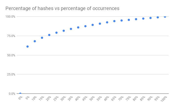
The first 5% of the hashes account for over 60% of occurrences! The first 5% provide the most value and only require a 47 MB bloom filter object. The first 10% of the hashes bumps that up to 68% of total occurrences for a 95 MB bloom filter. Each additional 5% of hashes has diminishing returns until roughly 40%. Depending on the requirements of the web application these small bloom filters can provide a lot of value.
Conclusions
Inserting the data set into a database is the best option. This provides 100% coverage, a 0% false positive rate, and extremely fast results. The draw back is this option requires a lot of disk storage, roughly 52 GB. If storing a large database is not an option, then a bloom filter is a great runner up. A bloom filter with 100% coverage and a 0.1% false positive rate requires ~945 MB of memory. Finally, if that is too much memory, 5% of the hashes results in a 47 MB bloom filter that covers 61% of the total occurrences.